The history of computing could arguably be divided into three eras: that of mainframes, minicomputers, and microcomputers. Minicomputers provided an important bridge between the first mainframes and the ubiquitous micros of today. This is the story of the PDP-11, the most influential and successful minicomputer ever.
In their moment, minicomputers were used in a variety of applications. They served as communications controllers, instrument controllers, large system pre-processors, desk calculators, and real-time data acquisition handlers. But they also laid the foundation for significant hardware architecture advances and contributed greatly to modern operating systems, programming languages, and interactive computing as we know them today.
In today’s world of computing, in which every computer runs some variant of Windows, Mac, or Linux, it’s hard to distinguish between the CPUs underneath the operating system. But there was a time when differences in CPU architecture were a big deal. The PDP-11 helps explain why that was the case.
The PDP-11 was introduced in 1970, a time when most computing was done on expensive GE, CDC, and IBM mainframes that few people had access to. There were no laptops, desktops, or personal computers. Programming was done by only a few companies, mostly in assembly, COBOL, and FORTRAN. Input was done on punched cards, and programs ran in non-interactive batch runs.
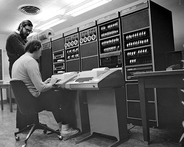
Although the first PDP-11 was modest, it laid the groundwork for an invasion of minicomputers that would make a new generation of computers more readily available, essentially creating a revolution in computing. The PDP-11 helped birth the UNIX operating system and the C programming language. It would also greatly influence the next generation of computer architectures. During the 22-year lifespan of the PDP-11—a tenure unheard of by today’s standards—more than 600,000 PDP-11s were sold.
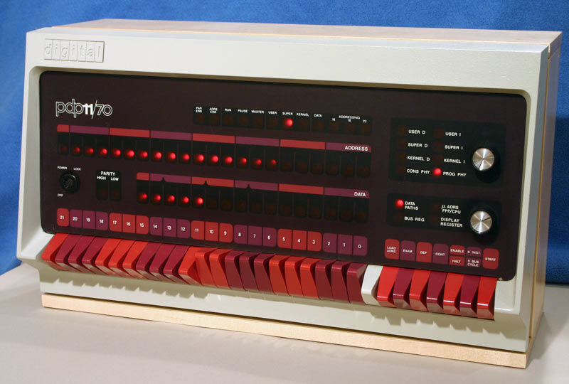
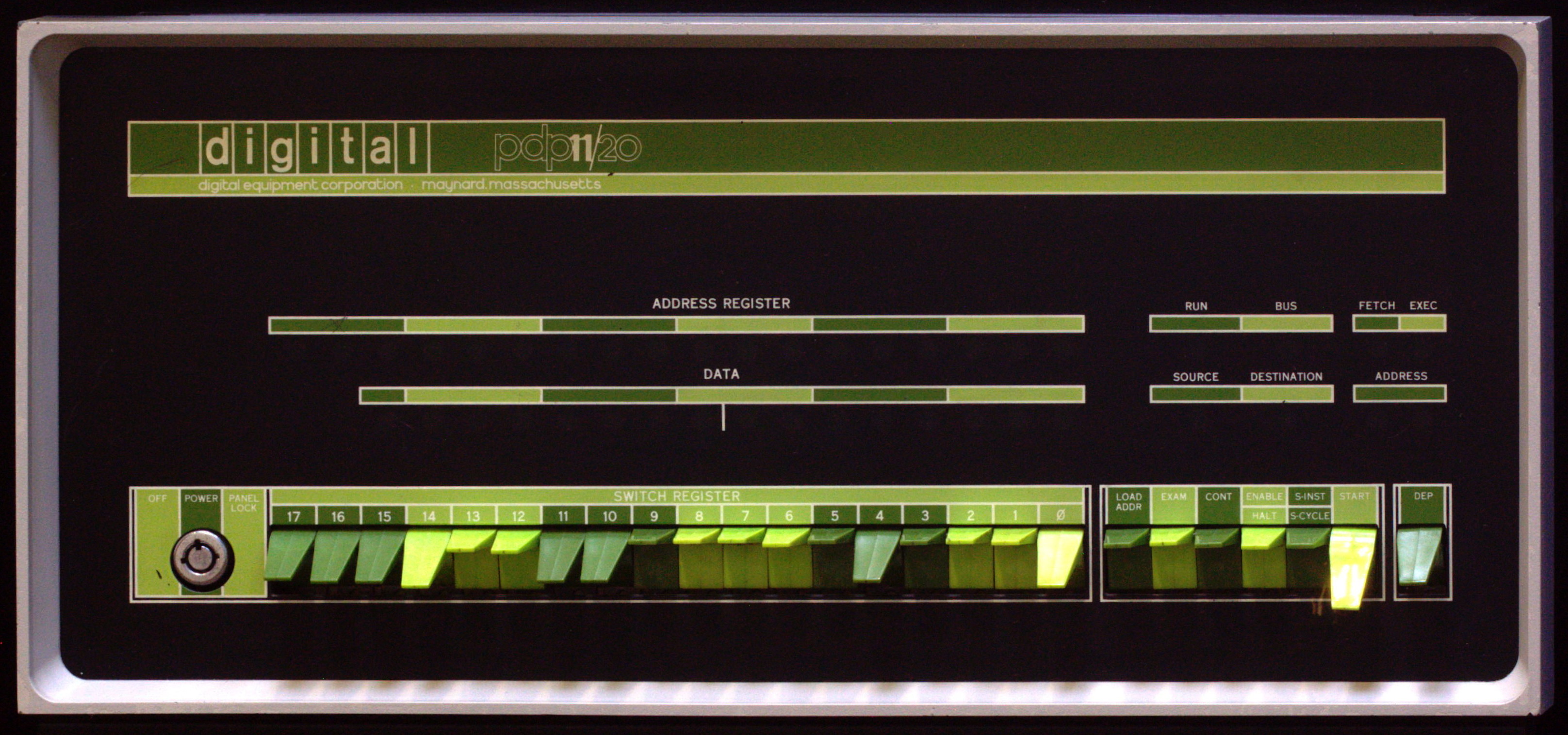
Early PDP-11 models were not overly impressive. The first PDP-11 11/20 cost $20,000, but it shipped with only about 4KB of RAM. It used paper tape as storage and had an ASR-33 teletype printer console that printed 10 characters per second. But it also had an amazing orthogonal 16-bit architecture, eight registers, 65KB of address space, a 1.25 MHz cycle time, and a flexible UNIBUS hardware bus that would support future hardware peripherals. This was a winning combination for its creator, Digital Equipment Corporation.
The initial application for the PDP-11 included real-time hardware control, factory automation, and data processing. As the PDP-11 gained a reputation for flexibility, programmability, and affordability, it saw use in traffic light control systems, the Nike missile defense system, air traffic control, nuclear power plants, Navy pilot training systems, and telecommunications. It also pioneered the word processing and data processing that we now take for granted.
And the PDP-11's influence is most strikingly evident in the device’s assembly programming.
Assembler programming basics
Before high-level languages such as Python, Java, and Fortran were invented, programming was done in assembly language. Assembly language programming can be done with very little RAM and storage—perfect for the environment of the early days of computing.
Assembly language is a low-level intermediary format that is converted to machine language that can then be run directly by the computer. It is low-level because you are directly manipulating aspects of the computer’s architecture. Simply put, assembly programming moves your data byte by byte through hardware registers and memory. What made programming the PDP-11 different was that the minicomputer's design was elegant. Every instruction had its place, and every instruction made sense.
A 16-bit address space meant that each register could directly address up to 64KB of RAM, with the top 4K reserved for memory-mapped input and output. PDP-11s could address a total of 128KB of RAM using register segments (more on this in a bit). So despite PDP-11 systems coming with only 4KB of RAM, they were still productive through the clever use of early programming techniques.
An assembly language program
It's easiest to grasp this concept through an example of a simple PDP-11 assembly language program, which we'll go through below. Keywords that start with a “.” are directives to the assembler. .globl exports a label as a symbol to the linker for use by the operating system. .text defines the start of the code segment. .data defines the start of a separate data segment. Keywords ending with a “:” are labels. Assembly programming uses labels to symbolically address memory. (Note: With the PDP-11 jargon and coding to come, any text after / is a comment.)
| Keywords | Translation |
| .globl _main | Export label _main as an entry point for the operating system to use |
| .text | Start of instruction segment where read-only code lives |
| _main: MOV VAL1, R0 | Copy the word value at memory location VAL1 into register 0 |
| ADD $10, R0 | Add 10 to the value in register 0 |
| MOV R0, VAL1 | Copy the value in register 0 to the memory location VAL1 |
| _.data | Start of data segment where read/writable data lives |
| VAL1: .word $100 | Reserve 2 bytes of storage to hold Val1, initialized to 100 |
Although numeric values can be used for memory addresses, the use of labels instead of hard-coded addresses makes it easier to program and makes the code relocatable in memory. This gives the operating system flexibility when running the code, ensuring each program is fast and efficient.
The .data assembler directive puts the data in a memory segment that's both readable and writable. The memory segment for code is read-only to prevent programming errors from corrupting the program and causing crashes. This separation of instructions from data on the PDP-11 is called "split instruction and data." In addition to adding stability, this feature also doubles the address space by enabling 64KB for code and 64KB for data—this was considered quite an innovation at the time. Accordingly, Intel’s X86 microcomputers later made extensive use of segments.
PDP-11 architecture
What about the PDP-11 made it better to program with? Its simple but powerful architecture.
Eight 16-bit registers were the heart of the instruction set architecture, or ISA. Six registers were general-purpose, one was the stack pointer, and one was the program counter. The registers could access any other register—as well as memory or direct data—using one of the six different addressing modes. Each register could perform logic, math, or test operations on a 16-bit word of data, an 8-bit byte of data, or access memory. A register could also read or write a 16-bit word of memory or an 8-bit byte of memory. Later versions of PDP-11s added registers to directly process floating-point numbers.
Here’s a look at some of those addressing modes:
/ Direct register address
MOV $1, R0 / Move the number 1 into register 0
/ Register indirect
MOV $1, (r0) / Move the number 1 into the memory pointed to by register 0
/ Auto-increment
MOV $1,(r0)+ / Move the number 1 into the memory pointed to by register 0, and increase the address in register 0 by 1 word
/ Auto-decrement
MOV $1,-(r0) / Decrement the address in register 1, then move the number 1 into the memory it points to
/ Index register
MOV $1, START(r0) / Move the number 1 into the address created by adding the contents of register 1 to the address of START
Stack pointer and program counter
As mentioned, the PDP-11 keeps instructions and code in separate memory segments. The stack pointer, or SP, helps you manage data memory, and the program counter, or PC, helps you manage the execution order of your code.
In the early days of computing, CPUs had a limited number of registers, so most operations were done in memory. Stacks and heaps were the ways that programmers managed data in memory. The Heap was generally used for global variables, data, and constants. The stack was used for the dynamic variables and data used in subroutines. Having a dedicated register for the stack was a real luxury for programmers and contributed to faster program execution. Programming today uses the modern technique of garbage collection to automate memory management. But in assembly language programming, if you need to use memory, you have to manage every aspect of it manually. Stack pointer instructions help you do that.
Here are stack pointer addressing modes.
/ Deferred
MOV (SP), R0 / Move the value of the memory pointed to by the stack pointer to register 0
/ Auto increment
MOV $1, (SP)+ / Move the value 1 into the memory pointed to by the stack pointer and increment the value of the stack pointer
/ Indexed
MOV ARRAYSTART(SP), R0 / Create and effective address by adding the value of ARRAYSTART to the value of the stack pointer, move the contents of that value into register 0
/ Index deferred
MOV @VAL1(SP), R1
Use of the program counter
The program counter can be accessed like any of the other registers, but doing so is not a good idea. On the PDP-11, the program counter stays busy keeping track of the next instruction in memory. The program counter is intended to support jump, branching, and other control flow instructions. The effect of the instruction JMP START has the same effect as MOV START,PC: to start executing code at location START.
The difference here is that using a JMP or branch instruction clearly indicates a change in your flow control, making it easier to read a program and trace the execution. Here is an example of unconditional jumps and branches:
JMP START / Jump to the address of START, which can be anywhere in the 16-bit memory address space.
This is also called a "long jump" because the effective address of “START” uses all 16 bits. A long jump is also an example of a direct address.
BR CALC / Branch to the offset address of CALC, forward up to 127 words or backward up to 128 words
This has the same effect as ADD CALC, PC, where CALC is an 8-bit value that can be negative.
The branch instruction is also called a "short jump" because you can’t jump as far. In this case, CALC is an indirect address that is relative to the current address as an offset. So, for instance, if CALC was a location 32 words later in memory, the equivalent instruction would be to add 32 words to the Program counter.
Why the need for a long and a short jump? One word: memory. The 16-bit address in the long jump uses an extra byte. In a program or operating system with a lot of branching, this can add up to a sizable fraction of your 8K of system RAM. This is another example of clever PDP-11 techniques to deal with limited memory.
Testing and branching
With the PDP-11, testing and branching instructions are fundamental to conditionals and looping.
Comparison, math, and logic instructions perform operations on data that result in an update to the condition code, or CC. The CC is a read-only register whose bits are set as a result of these operations. CC contains the Z (or zero) bit, the N (or negative) bit, the V (or overflow) bit, and the C (or carry) bit. Branches and jumps can be conditioned on the state of the CC after an operation that sets a bit value.
Here's an example:
CMP A,B / Compare A and B by subtracting B from A, and setting Z, N, V, C bits accordingly
BEQ OUT / If they are equal, short branch to location OUT
And here is the assembly language equivalent of the following loop:
For (i=j=0; i< 100; i++)
J = j+I;
CLR R0 / Clear, or initialize register 0 to zero
CLR R1 / Initialize register 1 to zero
AGAIN: / AGAIN is a memory label to this memory address
CMP R0, $100 / Compare register 0 to the value 100
BGT QUIT / If register 0 is greater than 100, branch to QUIT
ADD R0,R1 / Add register 0 to register 1
INC R0 / Add 1 to register 0
BR AGAIN / Branch to AGAIN
QUIT: / QUIT is a memory label to this memory address
TST can be used to check a single value:
TST A / This will set (set to 1) or clear (set to 0) the Z or N bits, depending on the data
And the PDP-11 has a full complement of conditional branch instructions, including but not limited to:
BEQ / Branch if the previous result is equal to zero, that is, if Z bit is set to 1
BNE / Branch if the previous result is not equal to zero, that is, if Z bit is clear.
BGT / Branch if the first operand is greater than the second
BGE / Branch if the first operand is greater than or equal to the second
BLT / Branch if the first operand is less than the second
BLE / Branch if the first operand is less than or equal to the second
Data operations
Let’s take a look at instructions for data operations:
MOV $1, R0 / Move the value 1 into register 0
MOV $1,VAL1 / Move the value 1 into the memory location VAL1
VAL1: .byte 0, 0 / Here’s how to allocate and initialize 2 bytes, or 1 word of space, with the address of VAL1. The assembler replaces the symbol VAL1 with its address in memory whenever it is referenced. The symbolic address can be relocated in memory by the linker when the program is linked into an executable.
ADD $1, R0 / Add the value 1 to the contents in register 0
ADD $1, VAL1 / Add the value 1 to the value in memory location VAL1
SUB $10, VAL1 / Subtract 10 from the value in memory local VAL1
In almost all comparison instructions, registers and memory locations can be used interchangeably. This gives the assembly programmer more freedom, and it's one less thing to keep track of manually. It is helpful to keep data in registers whenever possible, as every register instruction that replaces a memory address reduces the memory footprint and executes faster. These are the key advantages of assembly programming over high-level languages—assembler code always runs faster and uses less memory.
Two’s complement notation and negative numbers
The PDP-11 natively supported positive and negative numbers through 16-bit and 8-bit integers. Later models added floating-point registers. In two’s complement notation, if the highest bit is set...
| High | Low |
| 10000000 | 00000010 |
... then the number is considered negative. The number above represents -2.
In this way, the arithmetic logic unit (ALU) can add, subtract, multiply, and divide positive and negative integer numbers. The assembler makes using numbers easy. Just use a $ to represent a decimal number: Both $64 and $-1055 are valid numbers.
Traditionally, the PDP-11 used octal, or base 8 notation. Within this, 123 octal is the same as 83 base 10, or 1010011 in binary. Since we are programming under UNIX with the PDP-11, we use base 10.
Using subroutines
Let’s go deeper by working through some situations on a PDP-11. Say you're writing an assembler program and you have a piece of code you will use repeatedly from different parts of your program. Why not write a subroutine and call it from different parts of your program? The easy part is jumping to the start of your subroutine: JMP START.
The tricky part is getting back to where you called the subroutine. The old-fashioned way was to manually save your return address before you call the subroutine:
MOV PC, RET_ADDR / Save the address of the program counter into memory location RET_ADDR
... and then copy it back at the end of your subroutine:MOV RET_ADDR,PC.
But what if you have nested subroutine calls—that is, one subroutine calling another subroutine? The bookkeeping and complexity add up quickly, which could lead to unreliable and buggy code. The PDP-11 had a fix for this issue that eliminated the waste of time and memory: the JSR and RTS pair of instructions.
JSR PC,START / Jump to subroutine START, save the program counter value onto the stack
This instruction does several things. First, it pushes the value of the program counter, the current memory location of your code being executed, onto the stack and increments the stack pointer. Then it jumps to the address of START, the beginning of your subroutine. At the end of your subroutine, you execute the statement:
RTS PC / Return from subroutine, using PC
This pops the return memory address off the stack and copies the address into the program counter, thus jumping to the return address. These kinds of stack operations worked great for nested subroutines. You do have to coordinate your stack pop operations with the stack push operations, though, because one miss and you'll have a serious programming error.
Consider this example of a subroutine. Let’s say we want to convert from degrees Fahrenheit to degrees Celsius for 100 values using integer math:
/* The code in C */

Int I;

Int Val1[100];

For (i=0; i< 100; i++){

Val1[i] = FTOC(i);

}

Int FTOC(int i){

Return (((i-32)*5)/8)

}

/ Convert 0 – 100 from Fahrenheit to Celsius
CLR R1 / Initialize the degrees counter
AGAIN:
CMP $100, R1
BGTE QUIT / If register 1 is greater than or equal to 100, quit loop
PUSH R1 / Push degrees in F value onto stack, as a parameter for FTOC subroutine
JSR PC, FTOC / Call FTOC subroutine
POP R3 / Retrieve Centigrade temperature
MOV R3, VAL1(R1) / Copy Centigrade value to array in memory
INC R1 / Increment R1
BR AGAIN / Loop again
QUIT:
… / The rest of your program could go here
.end
FTOC: / Subroutine to convert degrees Fahrenheit to Celsius
POP R0
SUB 32,R0
MUL 5,R0
DIV 8,R0
Push R0
RTS PC
.data
VAL1: .WORD 100 / Our array of values
And here's another code example that shows the power of the auto increment deferred addressing mode. In this example, we're trying to implement the operation of a print buffer to efficiently move characters from one location in memory to another where they can be printed.
INIT:
MOV #SRC, R0 / Set up source address
MOV #BUFSTART, R1 / Set up destination address
MOV $76, R2 / Set up loop count with size of buffer
BEGIN:
MOVB (R0)+, (R1)+ / Move one character and increment both source and destination addresses
DEC R2 / Decrement count by one
BNE BEGIN / Loop back
… / The rest of the program
Using bigger numbers
When it comes to capacity, 16 bits can hold numbers up to 65,536. But what if you want to perform math on numbers larger than that? ADC and SBC come to the rescue.
MOV $65536, R0 / The highest value in 16 bits
ADD 1, R0 / The value 65537 is too large to hold in 16-bit two’s complement
ADC R1
In this case, when the bottom word of R0 overflows from the addition, ADC adds 1 to R1, effectively extending the number by another 16 bits, creating a 32-bit number. R1 is now bits 17 through 32 of this number, and more operations can be chained together to keep extending the range of the number. With a bit more work, you can support arbitrarily large integer numbers.
When using MUL to multiply numbers, the number of the destination register determines whether the multiplication is 16-bit or 32-bit. If the destination register is odd, the multiplication is 16-bit. If the destination register is even, the result is stored in both the registers. For instance:
MOV $32767, R0
MOV $10, R2
MUL R2,R0
System instructions and breakpoint traps
The PDP-11 has assorted other system instructions, including:
HALT / Halt the CPU
WAIT / Wait for an interrupt
RESET / Reset the external bus, including hardware device control and status registers
NOP / Do nothing ("No Operation")
And several instructions to support debugging:
TRAP / User invoked interrupt
BPT / Breakpoint trap
IOT / Input/output trap
RTI / Return from Interrupt
Trap instructions allow a computer to park whatever it is doing in a safe place, process something else, and then resume the original processing where it left off. This is useful for debugging or processing IO, priority system calls, or user-defined subroutines. The BPT and RIT instructions support the basics needed for building a debugger. ADB was the first UNIX debugger and is the direct predecessor of GDB, the powerful GNU debugger. ADB can set breakpoints, display values in registers and memory, set values, and single-step through code. Although sparse compared to GDB, it was a programmer’s best friend in the '70s and '80s.
How does debugging work at the machine code level? When the BPT instruction is run, the trap bit in the processor status register will direct the processor to a certain program address after executing each instruction. This allows the debugger to single-step through program memory one instruction at a time. It also allows you to set breakpoints in your code so you can run up to a label or subroutine and then stop to examine the values.
To try this on any UNIX or Linux program with ADB or GDB, start a program in the debugger: Adb a.out. And then single-step by typing :s. The CPU is using breakpoint instructions.
Hello, World
Here is a program that interacts with the operating system and uses system calls to write output:
/ Hello, World in PDP-11 Assembler

.text

      sys write; msg; 15 / call UNIX system call, write to print msg text

      sys exit

.data

msg:
We call the system write routine with the address of the "Hello, World" string, denoted as "msg." We use the .data assembler directive to tell the assembler that the address of msg is in the data segment.
The "Hello, World" text is defined as a sequence of bytes followed by a null character. Its memory location is defined by the label "msg." So we print the text by pushing the value of the program counter register onto the stack, pushing the address of the text onto the stack, and jumping to the address of the write routine. The write routine pops the address of the text off the stack and prints the text. The write routine returns to the caller’s address by executing the RTS instruction, which copies the return address of the stack into the program counter.
This is how subroutines are called and how many subroutines can be nested. It's also the underlying mechanism for how high-level languages nest subroutines.
Booting a PDP-11 simulator
To really understand what the PDP-11 was capable of, let’s run some of this code on a simulated PDP-11. SimH, an amazing computer simulator application, is a veritable time machine into computing’s past. It allows you to run in simulation the code of dozens of classic computers, including several types of PDP-11s. We will use SimH, scripts, and boot data to configure a PDP-11 running an early version of BSD UNIX. On this, we can compile and run some assembly program examples. This version of UNIX was popular with universities and was used to teach classes, such as PDP-11 Assembly Language. These instructions assume installation on Linux but can be adapted for other platforms. In fact, I’m running 2.11 BSD UNIX in SimH in Ubuntu Linux running in Windows. I’m using Oracle’s VM Virtual Box to run Ubuntu Linux under Windows and running SimH under Ubuntu.
We will be using Warner Losh’s SimH configuration for a PDP-11/93 system with 4MB of RAM, two RD54 disk drives, one TS11 tape drive, and a system console. Warner painstakingly recreated the boot media for the last and best UNIX on the last and best PDP-11 (he provides a detailed description of the UNIX boot process, too). This version of UNIX actually supports Ethernet, so an ambitious person could even put a simulated PDP-11 on the web.
Let’s start our configuration. First, boot into Ubuntu. Then, bring up the Terminal application to access the command line.
Build the latest version of SimH for PDP-11:
% mkdir simh
% cd simh
% sudo apt install make
% sudo apt install gcc
% wget http://simh.trailing-edge.com/sources/simhv311-0.zip
% unzip simhv311-0.zip
% make pdp11
% sudo cp BIN/pdp11 /usr/local/bin
Now retrieve and assemble the boot image for 2.11 BSD UNIX patch 195:
% sudo apt install git
% sudo apt install expect
% mkdir mk211bsd
% git clone https://github.com/bsdimp/mk211bsd
% cd mk211bsd/195
% wget https://www.tuhs.org/Archive/Distributions/UCB/2.11BSD-pl195.tar
% tar xvf 2.11BSD-pl195.tar
% gunzip *.gz
% perl mk211p195tape.pl
% expect 211bsd-195.expect #
Edit the last two lines of 211bsd-195.ini to remove the #
Start the simulator:
% pdp11 211bsd-195.ini
:
: ra(0,0)unix
: ^D
Login as root with no password:
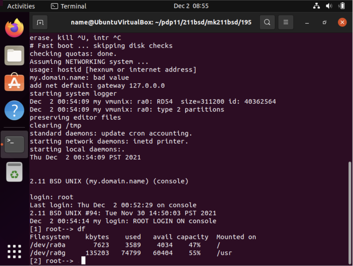
login: root
[1] root--> dfIf you made it this far, congratulations—you have assembled and booted into the last, best version of UNIX for the PDP-11, released in 1992.
Now that we have configured and booted into an emulated PDP-11 running classical UNIX, let’s write and run a basic assembly program.
First, get your backspace key to work by typing:
stty erase

Type the backspace key where it says . Then

mkdir coding

cd coding
Next, boost your tech street cred by running your antique version of the vi editor and create a makefile that compiles and links the program into an executable:
vi makefile


AS= /bin/as

SEPFLAG= -i -X

All: hw.as

hw: hw.o

        ld $(SEPFLAG) -o $@ /lib/crt0.o hw.o -lc

 key to end insert mode>
Next, type in your assembler program:
vi hw.as

i to insert text>

[assembly program goes here]

 >
Type "make" to compile and link your program. Now run your program by typing ./hw.
By writing and running code on a simulated PDP-11, you can relive the golden age of the minicomputer. Fifty years ago—before cell phones, before personal computers, before bitmapped screens and mice—this is how you wrote code.
The legacies: PDP-11, UNIX, and C
Most importantly, UNIX provided an interactive, time-shared system that was accessible from inexpensive terminals. PDP-11 with UNIX opened the floodgates for inexpensive interactive computing, which then led to an explosion of office productivity. People finally had a means of editing, storing, and printing office documents. This was big in the corporate world, obviously, but things were just getting started.
In 1977, a computer scientist named John Lions wrote one of the most famous computing books of all time: A Commentary on the UNIX Operating System. It contained an annotated, line-by-line description of the Unix kernel system code. The book was wildly popular until ATT’s lawyers clamped down on its publication. (Today, a legal copy of this book can be found here. If you want a detailed description of historical Unix kernel functionality, look no further.)
The C programming language was written by the same people writing Unix, and it descended from the BCPL language, which was itself a descendent of Algol. C evolved to take advantage of PDP-11 instruction set. The following C features compiled directly to the PDP-11 architecture:
- The ? operator is a direct equivalent of TST instruction
- The arithmetic and logic operators are direct equivalents to PDP-11 instructions
- Bit Operations compile to byte data operations
- Pointers for memory addressing are direct equivalents
Although the ++ and – operators in C are equivalents of DEC and INC instructions, they were inspired by an addressing mode in the PDP-7.
By the summer of 1973, the C language was mature enough to compile Unix, resulting in a virtuous cycle of productivity. Programming Unix in C allowed the development of Unix to accelerate, which led to more Unix features for people to use, which led to the sale of more PDP-11 systems in research, industry, manufacturing, and academia. That, in turn, resulted in larger, faster PDP-11 systems that enabled more Unix features.
C was a major advancement; it was a language that was portable across CPUs and could generate efficient operating system code. C’s success led to Objective C on the Mac, which led to today’s Swift. Bell Labs took C and created C++. Sun Microsystems took C++ and created Java. Microsoft took Java and created C# and wrote .NET with it. Other languages derived from C include JavaScript, TypeScript, Go, and Rust.
But most notably, ATT Unix led to BSD Unix, which led to MacOS and then iOS. (ATT Unix also led to Linux and GNU, which led to RedHat, Ubuntu, SUSE, Debian, Gentoo, Slackware, and other source distributions.)
Hopefully, this introduction to the PDP-11, its architecture, and how it is programmed gives you a better understanding of how and why computing progressed beyond non-interactive batch computing. Put simply, the PDP-11 helped popularize the interactive computing paradigm we take for granted today. If you’re looking for a single device that best represents the minicomputer lineage, the PDP-11 is it.
Further reading
For anyone wishing to delve deeper, Professor Eduard Desautels has graciously agreed to open-source his textbook Assembly Language Programming for PDP-11 and LSI-11 Computers, a book that was widely used in universities to introduce students to programming PDP-11 assembly. For many of us, it was our introduction to a new realm of "close to the metal" programming and a gateway to better understanding future computer architectures. It is arguably one of the best books on the subject. You can check out a PDF version of the book here: Assembly Language Programming for PDP-11.
Technology - Latest - Google News
March 14, 2022 at 06:45PM
https://ift.tt/T2pbZED
A brief tour of the PDP-11, the most influential minicomputer of all time - Ars Technica
Technology - Latest - Google News
https://ift.tt/ocbWhDr
https://ift.tt/gFw9U5a


0 Commentaires